The SQL language is already an old acquaintance of developers, database users and system administrators. It has been with us since 1974 and gives us the possibility of interacting with Relational Database Management Systems (RDBMS).
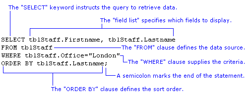
Geospatial SQL is an SQL specialization. It enables defining and manipulating relational data using the traditional INSERT/SELECT/UPDATE/DELETE operations. However, there are two fundamental differences that make geospatial SQL comprehensive enough to study it separately:
-
It works with spatial data, such as geometrics (points, lines, polygons, etc.) and raster data (representations of space in the form of a matrix of cells, each of which contains a distinctive value, such as an RGB color component in the case of images, a height in the case of an elevation map, a temperature, etc.).
- It allows the study of the spatial relationships between the mentioned data types.
Spatial relationships
The characteristic that is most special about geospatial SQL is therefore the ability to work with spatial relationships. The Open Geospatial Consortium is in charge of systemizing and classifying the relationships between geometric elements, thereby defining the Dimensionally Extended nine-Intersection Model (DE-9IM). This model defines the relationships that can occur between two geometric regions (the relationships with raster data are more recent and still lack specifications as well-defined as these) in a bi-dimensional (2D) environment, taking into account that:
-
All geometric elements in 2D have 3 distinctive parts: the edge, the interior and the exterior.
-
There are 3 types of elements that can be related in a 2D space: points (dimension 0), lines (dimension 1) and polygons (dimension 2)
The problem with this model is that it is too complex for practical use. Therefore, to make it usable, a series of predicates were defined and implemented in spatial database managers , such as PostGIS. The arguments used by these predicates are two regions in the 2D space from which they return a result of TRUE (the predicate is always fulfilled) or FALSE (the predicate is not fulfilled). The basic predicates are:
-
Contains (regionA, regionB): If region B is contained in region A, this predicate returns TRUE. Otherwise, it returns FALSE. We highlight in to differentiate this predicate from the Covers predicate, which will be explained further along.
-
Disjoints (regionA, regionB): If regions A and B do not share any points, it returns TRUE. Otherwise, it returns FALSE. This predicate is the opposite of Intersects, which will be explained further along.
-
Touches (regionA, regionB): If both regions share any edges, but have no interior points in common, this predicate returns TRUE. Otherwise, it returns FALSE.
-
Equals (regionA, regionB): If both regions are topologically the same; that is, if both their limits match, this predicate returns TRUE. Otherwise, it returns FALSE. Note that Equals => Contains
-
Crosses (regionA, regionB): If both regions share any interior points, but not all, this predicate returns TRUE. Otherwise, it returns FALSE.
-
Overlaps (regionA, regionB): If both regions share 2D space, both geometrics are of the same dimension and one does not completely contain the other one, this predicate returns TRUE. Otherwise, it returns FALSE.
There is another series of predicates that derives from these and is also frequent:
-
Within (regionB, regionA) = Contains(regionA, regionB)
-
Intersects (regionA, regionB) = NOT Disjoints(regionA, regionB)
-
Intersects (regionA, regionB) = Overlaps(regionA, regionB) OR Touches(regionA, regionB) OR Contains(regionA, regionB)
-
Covers (regionA, regionB) = If none of the points of region B are outside region A.
For a proper understanding of predicates at this point, certain subtle differences have to be taken into account; there are some predicates that are very similar, but differ in the level of restriction they apply to return TRUE:
-
Overlaps can be considered a more restrictive version of Intersects. Overlaps requires both regions to be of the same dimension and that one not completely contain the other. Other than that, the predicates are the same.
-
Covers and Contains are also a more restrictive version of the other predicate. This is clearly seen in the image below:
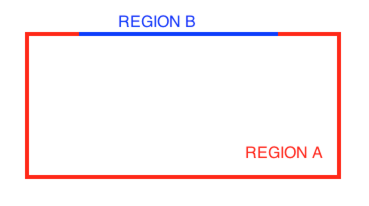
In this situation, the result of both predicates would be:
-
Contains (REGION A, REGION B) = FALSE
-
Covers (REGION A, REGION B) = TRUE
This is because Contains is more restrictive than Covers. Contains requires at least one point of the interior of B to be in the interior of A. In this case, all B points are on the edge of A and none in its interior.
In our case, we are especially interested in learning the implementation performed in PostGIS. PostGIS is the spatial extension of the PostgreSQL database. Both PostgreSQL and PostGIS have an Open Source license and are free. They also share a high degree of maturity and are backed by an immense community of users. That is why it is particularly easy to access them and start to experiment with geospatial SQL. Both tools have installers for Windows, Linux and Mac OS systems. Furthermore, for those who prefer to experiment with the language, without installing anything on their equipment, there is always CartoDB. Simply sign up to get your free account, which lets you create up to 5 tables and run SQL queries in a matter of minutes.
Spatial indexes
We end this introduction by noting that there is another essential component that can be used with geospatial SQL: the spatial index.
These indexes are well known in relational database circles. They are data structures used for faster access to database records. They do so simply by storing the most frequently used entries in the table in a rapid-access memory area.
The problem with spatial databases is that the traditional indexes do not work well with the types of operations that might interest us, such as obtaining the points closest to a location, calculating the distance between points or finding out whether a polygon intersects with another polygon or not. This is why the data tables that contain columns with special features usually generate spatial indexes that allow queries to be run several times more quickly.
In later posts, we will explain geospatial SQL in more detail, with specific examples, such as the use of raster data along with geometric data.


